Heat Exchangers MIT thermodynamics notes
http://web.mit.edu/16.unified/www/FALL/thermodynamics/notes/node131.html#18481

The general function of a heat exchanger is to transfer heat from one fluid to another. The basic component of a heat exchanger can be viewed as a tube with one fluid running through it and another fluid flowing by on the outside. There are thus three heat transfer operations that need to be described:
Here we have taken into account one additional thermal resistance than in Section 17.2, the resistance due to convection on the interior, and include in our expression for heat transfer the bulk temperature of the fluid, TA , rather than the interior wall temperature, T1 .
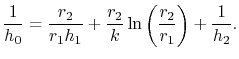
From (18.21) and (18.22) the overall heat transfer coefficient, h0 , is
We will make use of this in what follows.
To address this we start by considering the general case of axial variation of temperature in a tube with wall at uniform temperature T0 and a fluid flowing inside the tube (Figure 18.12).
 where D is the pipe diameter. The heat given to the fluid (the change in enthalpy) is given by
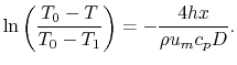
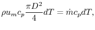 where rhois the density of the fluid, um is the mean velocity of the fluid,cp is the specific heat of the fluid and m is the mass flow rate of the fluid. Setting the last two expressions equal and integrating from the start of the pipe, we find
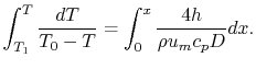 Carrying out the integration,
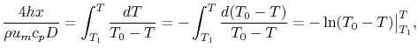 i.e.,
i.e.,
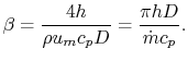
Equation (18.24) can be written as
 where
where
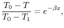
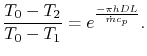
 This is the temperature distribution along the pipe. The exit temperature at x=L is
The total heat transfer to the wall all along the pipe is
From Equation (18.25),
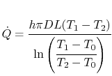
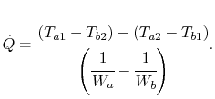
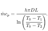 The total rate of heat transfer is therefore
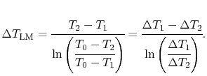
where DTLM is the logarithmic mean temperature difference, defined as
The concept of a logarithmic mean temperature difference is useful in the analysis of heat exchangers. We will define a logarithmic mean temperature difference for the general counterflow heat exchanger below.
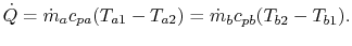
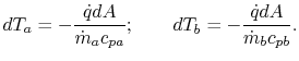
 From a local heat balance, the heat given up by stream a in length dx is (There is a negative sign since Ta decreases). The heat taken up by stream b is
  . (There is a negative sign because Tb decreases as x increases). The local heat balance is
Solving (18.29) for dTa and dTb, we find
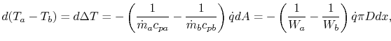 where
where  . Also,
  where h0 is the overall heat transfer coefficient. We can then say
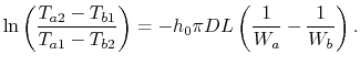
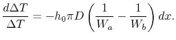 Integrating from x=o to x=L gives
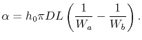
Equation (18.30) can also be written as
where
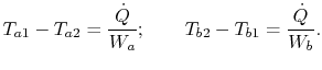
 We know that
Thus
 Solving for the total heat transfer:
Rearranging (18.30) allows us to express  in terms of other parameters as
Substituting (18.34) into (18.33) we obtain a final expression for the total heat transfer for a counterflow heat exchanger:
This is the generalization (for non-uniform wall temperature) of our result from Section 18.5.1.
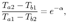
Eliminating Q from (18.32),
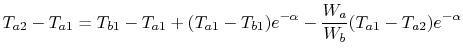
We now have two equations, (18.37) and (18.38), and two unknowns, Ta2 and Tb2. Solving first for Ta2,
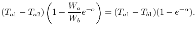 or
or
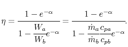
where n is the efficiency of a counterflow heat exchanger:
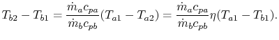
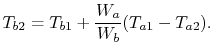
Equation 18.39 gives Ta2 in terms of known quantities. We can use this result in (18.38) to find Tb2:
 We examine three examples.

The general function of a heat exchanger is to transfer heat from one fluid to another. The basic component of a heat exchanger can be viewed as a tube with one fluid running through it and another fluid flowing by on the outside. There are thus three heat transfer operations that need to be described:
- Convective heat transfer from fluid to the inner wall of the tube,
- Conductive heat transfer through the tube wall, and
- Convective heat transfer from the outer tube wall to the outside fluid.
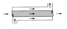
Heat exchangers are typically classified according to flow arrangement and type of construction. The simplest heat exchanger is one for which the hot and cold fluids move in the same or opposite directions in a concentric tube (or double-pipe) construction. In the parallel-flow arrangement of Figure 18.8(a), the hot and cold fluids enter at the same end, flow in the same direction, and leave at the same end. In the counterflow arrangement of Figure 18.8(b), the fluids enter at opposite ends, flow in opposite directions, and leave at opposite ends.
 [Counterflow]
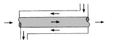
[Finned with both fluids unmixed.]
 [Unfinned with one fluid mixed and the other unmixed] [Unfinned with one fluid mixed and the other unmixed] 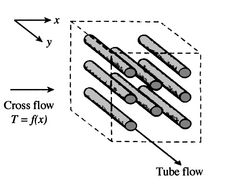 |
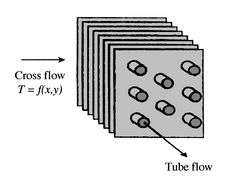
Alternatively, the fluids may be in cross flow (perpendicular to each other), as shown by the finned and unfinned tubular heat exchangers of Figure 18.9. The two configurations differ according to whether the fluid moving over the tubes is unmixed or mixed. In Figure 18.9(a), the fluid is said to be unmixed because the fins prevent motion in a direction ( y) that is transverse to the main flow direction ( x). In this case the fluid temperature varies with x and y . In contrast, for the unfinned tube bundle of Figure 18.9(b), fluid motion, hence mixing, in the transverse direction is possible, and temperature variations are primarily in the main flow direction. Since the tube flow is unmixed, both fluids are unmixed in the finned exchanger, while one fluid is mixed and the other unmixed in the unfinned exchanger.
To develop the methodology for heat exchanger analysis and design, we look at the problem of heat transfer from a fluid inside a tube to another fluid outside.
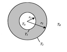
We examined this problem before in Section 17.2 and found that the heat transfer rate per unit length is given by
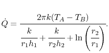
It is useful to define an overall heat transfer coefficient h0 per unit length as
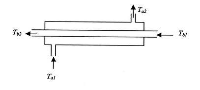
A schematic of a counterflow heat exchanger is shown in Figure 18.11. We wish to know the temperature distribution along the tube and the amount of heat transferred.
18.5.1 Simplified Counterflow Heat Exchanger (With Uniform Wall Temperature)
To address this we start by considering the general case of axial variation of temperature in a tube with wall at uniform temperature T0 and a fluid flowing inside the tube (Figure 18.12).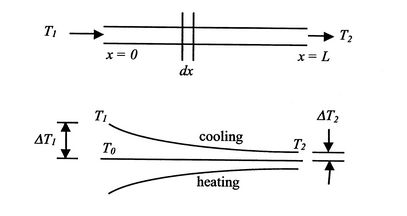
The objective is to find the mean temperature of the fluid at x ,T(x) , in the case where fluid comes in at x=0 with temperature T1 and leaves at x=L with temperature T2. The expected distribution for heating and cooling are sketched in Figure 18.12.
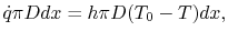
For heating (T0 >T ), the heat flow from the pipe wall in a length dx is
 | |
or | |
| (18..27) | |
18.5.2 General Counterflow Heat Exchanger
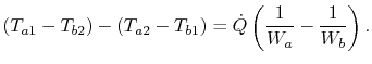
We return to our original problem, to Figure 18.11, and write an overall heat balance between the two counterflowing streams as
 in terms of other parameters as
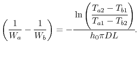
| Q | 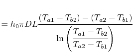 | (18..35) |
or | ||
| Q | (18..36) | |
18.5.3 Efficiency of a Counterflow Heat Exchanger
Suppose we know only the two inlet temperatures Ta1, Tb1, and we need to find the outlet temperatures. From (18.31),
or, rearranging, | ||
| (18..37) | ||
 DT can approach zero at cold end.
n _==>1 as h0 , surface area,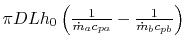 .
.
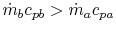
Maximum value of ratio
Maximum value of ratio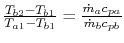 .
.
 a is negative,n
 as
as ![$ [\;]\rightarrow\infty\;(W_b < W_a)$](http://web.mit.edu/16.unified/www/FALL/thermodynamics/notes/img2222.png)
Maximum value of ratio
Maximum value of ratio .
.
temperature difference remains uniform, n=1 .

Commenti
Posta un commento